Simple Fuzzy Logic Controller
Background
This FLC was
originally designed to provide the simplest Fuzzy Logic controller possible in
MS VC++.
For details on
FL, two good e-books are available on the Internet:
- “Fuzzy Control,” Kevin M. Passino and Stephen
Yurkovich, Addison Wesley Longman,
- “Fuzzy Logic: a Practical Approach,” McNeill,
Martin and Ellen Thro., 1994 Academic Press
Professional.
http://www.fuzzysys.com/books/FLLib/FUZZYPDF/FUZZYLOG.PDF
Also, this FLC
has been implemented in accordance with the Seattle Robotics “practical”
tutorial on the topic:
http://www.seattlerobotics.org/encoder/mar98/fuz/flindex.html
It is therefore
highly recommended to read it to understand this implementation.
Pre-requisite
The program uses a simple 2D chart ActiveX component. It is called NTGraph.OCX, and is usually placed in the C:\WINDOWS\System32 system folder. The component must be registered before it can be used: “regsvr32 C:\WINDOWS\System32\NTGraph.ocx”
This can be done simply from the “Start – Run” command line, or type CMD to open a DOS-like window.
This is a quick user guide; a separate FL design guide will follow.
Quick Program Description
User interface

Note: The underlying classes are more versatile than this dialog based example can show.
In this implementation, the FLC is limited to 3 fuzzy variables: 2 inputs and 1 output.
FL Design
The design has been simplified so that future implementations of complex fuzzy systems remain feasible. Basically a Fuzzy Controller is an object consisting of 3 main components:
The first component is a collection of Fuzzy Sets (FS). In a nutshell, a Fuzzy Set is itself a collection of Membership Functions representing common fuzzy states, like “Low”, “Average”, “High” or “Negative”, “Null”, “Positive”. Semantically, a fuzzy set is linked to the variable it will be associated with, but it is a separate object nonetheless.
The second component is a collection of fuzzy variables (VS). The object model allows for any number of variables, but this implementation assumes 2 inputs and 1 output. As said above, each variable is associated to a fuzzy set.
The last component is the Rule Set (RS).
The model allows for complex rules like:
IF Var1 is High OR Var2 is Low AND Var3 is Average THEN Var4 is Average
Note that rules are interpreted sequentially, i.e. the above rule is equivalent to:
IF (Var1 is High OR Var2 is Low) AND Var3 is Average THEN Var4 is Average
In the current implementation, the FLC uses 3 variables: 2 inputs and 1 output, all associated with a Fuzzy Set consisting of 3 Fuzzy States. The Rule Set is completely defined with a 3 x 3 rule matrix.
Starting…
A new FLC object is instantiated when the dialog is loaded. The FLC is empty, i.e. it has no FS, no VS and no RS. It is therefore necessary to create them first.
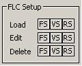 Note that these
buttons instantiate the necessary appropriate objects, and load default values
as per the Seattle
Robotics tutorial, the only difference being that data is normalised in
this implementation. The FLC can only
operate when its 3 main components are loaded.
Note that these
buttons instantiate the necessary appropriate objects, and load default values
as per the Seattle
Robotics tutorial, the only difference being that data is normalised in
this implementation. The FLC can only
operate when its 3 main components are loaded.
The FLC status list box at the bottom of the form displays the FL process.
Note: Input data must be normalised to the [-1; +1] range, the output will also range from -1 to +1.
FS Editor
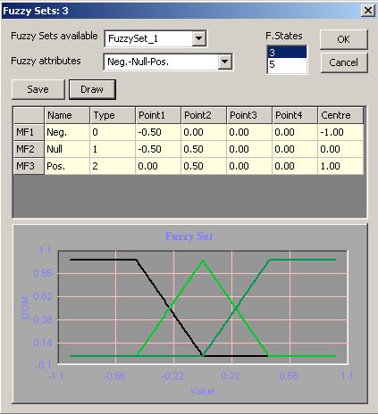
In the current implementation, only 3 types of membership functions have been coded: Shoulder-Right (black line above), Triangle (green), and Shoulder-Left (dark green). That should suffice for most situations.
It is not here permitted to change the number of fuzzy states, but one could theoretically delete the fuzzy sets, create new ones, or just leave the FS unused. The underlying classes allow that.
As a reminder, a DOM (Degree of Membership) can be calculated for each state. For instance, when Value = 0.25, DOM(Neg.) = 0, DOM(Null) = 0.5, and DOM(Pos.) = 0.5
Changes to the grid are applied to the Fuzzy Set when the “Save” button is pressed.
VS Editor
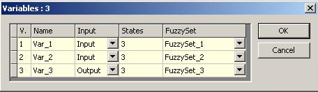
This dialog is quite simple. A variable can only be an input or an output, and a fuzzy set is associated to each variable.
Variable names can be changed. The Number of States is read-only in this version, but a Fuzzy Set can be dropped, or changed.
Please note that a Fuzzy Set attached to a Variable is copied into it. Subsequent changes to the Fuzzy Set are not reflected to the variable until a new association is effected.
RS Editor
As said before, rules could be complex,
using different fuzzy Boolean operators on more than 2 premises. In our implementation, rules are made of 2
premises and 1 consequent, and the Boolean operator is a fuzzy
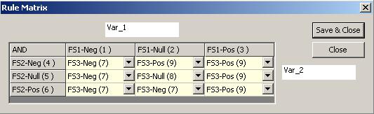
In the dialog above, the rules are all of the same format:
IF Var_1 is XXX AND Var_2 is YYY then Var_3 is ZZZ
Where XXX is a fuzzy state defined in FS1 (attached to Var_1), etc…
For instance, the top left cell is:
IF Var_1 is “FS1-Neg” AND Var_2 is “FS2-Neg” THEN Output is “FS3-Neg”
The premises number are now also displayed so the rule can also be read as:
If 1 AND 4 THEN 7
This makes rule handling easier.
The rule matrix is here fully defined and symmetrical, as often is the case.
Again, rules use premises in the form of an association of variables with a fuzzy state. A rule set therefore closely depends on the variable set, and again subsequent changes to fuzzy sets are not reflected in the Variable Set, or in the Rule Set.
Note: strictly speaking, a rule follows the
format:
IF Premise THEN Consequent,
a premise being composed of one or several antecedents. In our model, for simplicity’s sake, each
antecedent is called a premise. This
does not compromise calculations at all.
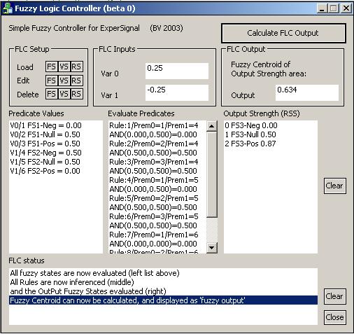
Calculating a Fuzzy Output
FS, VS and RS are defined, so we can now start calculating fuzzy outputs.
There are 3 stages in this process:
1) Calculate Predicate Values
V0 is the 1st variable. It
has been associated to Fuzzy Set FS1, and each fuzzy state is evaluated.
At the same time, a premise number is already given, to simplify rule
processing later on: “V0 is FS1-Neg” is Premise 1, “V0 is FS1-Null” is Premise
2, and so on…
2) Evaluate Predicates
Each rule is now evaluated. Since premises are already indexed, this
process is quite straightforward.
In the example above, Rule 1 is composed of Prem0 = 1 and Prem1 = 4 and a Fuzzy
AND is applied to them (using the common Min-Max convention).
3) Output Strength
After a single rule scan, the Output can now be
calculated for each of its fuzzy states
4) “Defuzzification”
The Fuzzy centroid is calculated using the Root-Sum-Square Method, which is one
of the most balanced methods. It is also
theoretically possible to inhibit or cap specific rule or rules. The Seattle
Robotics provides ample information on this if needed.
Conclusion
This is a very basic implementation of an interesting object model. FLC can now be easily assembled into more complex problem solving tools.
A derived class will now be used to implement sequences, etc in a State Machine model still under consideration.
It is also possible to now add a data input module (file read) and apply Genetic Algorithms to optimise some or all of the FLC components. Some experimentations of mine (using Ward’s GeneHunter) will be released soon.
As always, feedback and comments of all sorts most welcome…
bruno
Appendix
Here is one sample calculation taken from the Seattle Robotics tutorial
Inputs:
Var_0 = -0.25 (normalised to [-1;+1])
Var_1 = -.25 (normalised to [-1;+1])
Output:
Output = -0.635 (using Fuzzy Centroïd method)
Now, let’s do the same with our Simple FLC:
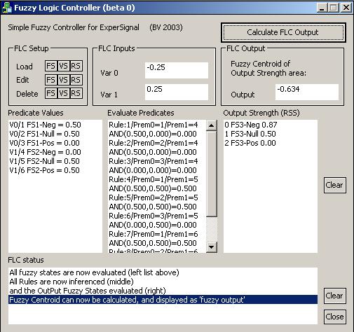
Output = -0.634
Note: The default Fuzzy Sets and Rule Sets conform the tutorial examples.
Voilà! J